Demo - Fairness Analysis of COMPAS by ProPublica
Based on: https://github.com/propublica/compas-analysis
What follows are the calculations performed for ProPublica’s analaysis of the COMPAS Recidivism Risk Scores. It might be helpful to open the methodology in another tab to understand the following.
import numpy as np
import pandas as pd
from scipy import stats
import matplotlib.pylab as plt
import seaborn as sns

from responsibly.dataset import COMPASDataset
from responsibly.fairness.metrics import distplot_by
Loading the Data
We select fields for severity of charge, number of priors, demographics, age, sex, compas scores, and whether each person was accused of a crime within two years.
There are a number of reasons remove rows because of missing data:
If the charge date of a defendants Compas scored crime was not within 30 days from when the person was arrested, we assume that because of data quality reasons, that we do not have the right offense.
We coded the recidivist flag –
is_recid– to be -1 if we could not find a compas case at all.In a similar vein, ordinary traffic offenses – those with a
c_charge_degreeof ‘O’ – will not result in Jail time are removed (only two of them).We filtered the underlying data from Broward county to include only those rows representing people who had either recidivated in two years, or had at least two years outside of a correctional facility.
All of this is already done by instantiating a COMPASDataset object
from responsibly.
compas_ds = COMPASDataset()
df = compas_ds.df

len(df)
6172
EDA
Higher COMPAS scores are slightly correlated with a longer length of stay.
stats.pearsonr(df['length_of_stay'].astype(int), df['decile_score'])
(0.20741201943031584, 5.943991686971499e-61)
After filtering we have the following demographic breakdown:
df['age_cat'].value_counts()
25 - 45            3532
Less than 25       1347
Greater than 45    1293
Name: age_cat, dtype: int64
df['race'].value_counts()
African-American    3175
Caucasian           2103
Hispanic             509
Other                343
Asian                 31
Native American       11
Name: race, dtype: int64
(((df['race'].value_counts() / len(df))
  * 100)
 .round(2))
African-American    51.44
Caucasian           34.07
Hispanic             8.25
Other                5.56
Asian                0.50
Native American      0.18
Name: race, dtype: float64
df['score_text'].value_counts()
Low       3421
Medium    1607
High      1144
Name: score_text, dtype: int64
pd.crosstab(df['sex'], df['race'])
| race | African-American | Asian | Caucasian | Hispanic | Native American | Other |
|---|---|---|---|---|---|---|
| sex | ||||||
| Female | 549 | 2 | 482 | 82 | 2 | 58 |
| Male | 2626 | 29 | 1621 | 427 | 9 | 285 |
(((df['sex'].value_counts() / len(df))
  * 100)
 .round(2))
Male      80.96
Female    19.04
Name: sex, dtype: float64
df['two_year_recid'].value_counts()
0    3363
1    2809
Name: two_year_recid, dtype: int64
(((df['two_year_recid'].value_counts() / len(df))
  * 100)
 .round(2))
0    54.49
1    45.51
Name: two_year_recid, dtype: float64
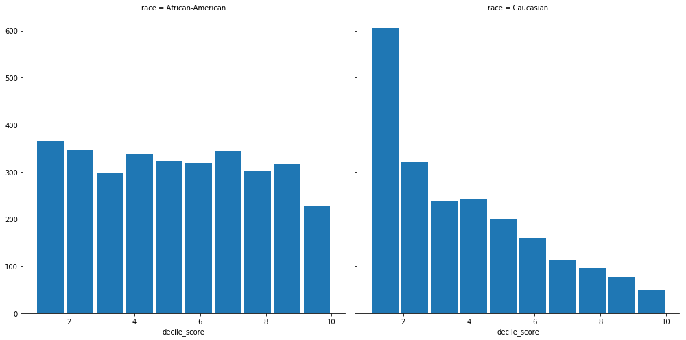
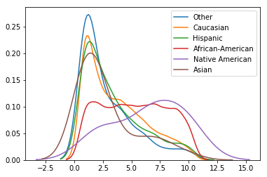
Judges are often presented with two sets of scores from the Compas system – one that classifies people into High, Medium and Low risk, and a corresponding decile score. There is a clear downward trend in the decile scores as those scores increase for white defendants.
RACE_IN_FOCUS = ['African-American', 'Caucasian']
df_race_focused = df[df['race'].isin(RACE_IN_FOCUS)]
g = sns.FacetGrid(df_race_focused, col='race', height=7)#, aspect=4,)
g.map(plt.hist, 'decile_score', rwidth=0.9);
distplot_by(df['decile_score'], df['race'], hist=False);
pd.crosstab(df['decile_score'], df['race'])
| race | African-American | Asian | Caucasian | Hispanic | Native American | Other |
|---|---|---|---|---|---|---|
| decile_score | ||||||
| 1 | 365 | 15 | 605 | 159 | 0 | 142 |
| 2 | 346 | 4 | 321 | 89 | 2 | 60 |
| 3 | 298 | 5 | 238 | 73 | 1 | 32 |
| 4 | 337 | 0 | 243 | 47 | 0 | 39 |
| 5 | 323 | 1 | 200 | 39 | 0 | 19 |
| 6 | 318 | 2 | 160 | 27 | 2 | 20 |
| 7 | 343 | 1 | 113 | 28 | 2 | 9 |
| 8 | 301 | 2 | 96 | 14 | 0 | 7 |
| 9 | 317 | 0 | 77 | 17 | 2 | 7 |
| 10 | 227 | 1 | 50 | 16 | 2 | 8 |
pd.crosstab(df['two_year_recid'], df['race'], normalize='index')
| race | African-American | Asian | Caucasian | Hispanic | Native American | Other |
|---|---|---|---|---|---|---|
| two_year_recid | ||||||
| 0 | 0.450193 | 0.006839 | 0.380910 | 0.095153 | 0.001784 | 0.065120 |
| 1 | 0.591314 | 0.002848 | 0.292631 | 0.067284 | 0.001780 | 0.044144 |
pd.crosstab(df_race_focused['two_year_recid'],
            df_race_focused['race'],
            normalize='index')
| race | African-American | Caucasian |
|---|---|---|
| two_year_recid | ||
| 0 | 0.541682 | 0.458318 |
| 1 | 0.668949 | 0.331051 |
Fairness Demographic Classification Criteria
Based on: https://fairmlbook.org/demographic.html
from responsibly.fairness.metrics import (independence_binary,
                                        separation_binary,
                                        sufficiency_binary,
                                        independence_score,
                                        separation_score,
                                        sufficiency_score,
                                        report_binary,
                                        plot_roc_by_attr)
Independence
indp, indp_cmp = independence_binary((df_race_focused['decile_score'] > 4),
                                     df_race_focused['race'],
                                     'Caucasian',
                                     as_df=True)
indp, indp_cmp = independence_binary((df_race_focused['decile_score'] > 4),
                                     df_race_focused['race'],
                                     'Caucasian',
                                     as_df=True)
indp.plot(kind='bar');
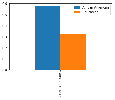
indp_cmp
| acceptance_rate | |
|---|---|
| African-American vs. Caucasian | |
| diff | 0.245107 |
| ratio | 1.740604 |
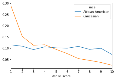
independence_score(df_race_focused['decile_score'],
                   df_race_focused['race'], as_df=True).plot();
Separation
sep, sep_cmp = separation_binary(df_race_focused['two_year_recid'],
                                 (df_race_focused['decile_score'] > 4),
                                 df_race_focused['race'],
                                 'Caucasian',
                                as_df=True)
sep.plot(kind='bar');
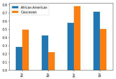
sep_cmp
| fnr | fpr | tnr | tpr | |
|---|---|---|---|---|
| African-American vs. Caucasian | ||||
| diff | -0.211582 | 0.203241 | -0.203241 | 0.211582 |
| ratio | 0.573724 | 1.923234 | 0.739387 | 1.420098 |
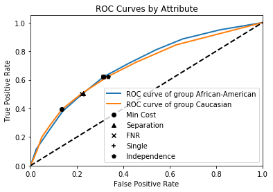
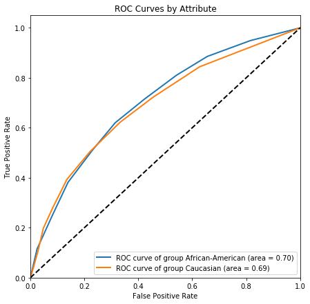
plot_roc_by_attr(df_race_focused['two_year_recid'],
                 df_race_focused['decile_score'],
                 df_race_focused['race'],
                 figsize=(7, 7));
Sufficiency
suff, suff_cmp = sufficiency_binary(df_race_focused['two_year_recid'],
                                   (df_race_focused['decile_score'] > 4),
                                   df_race_focused['race'],
                                   'Caucasian',
                                   as_df=True)
suff.plot(kind='bar');
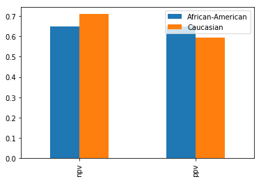
suff_cmp
| npv | ppv | |
|---|---|---|
| African-American vs. Caucasian | ||
| diff | -0.061433 | 0.054708 |
| ratio | 0.913477 | 1.091972 |
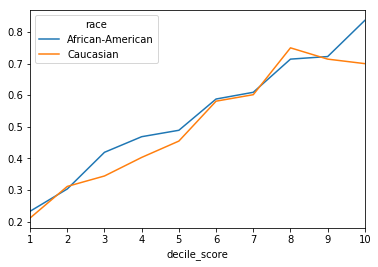
sufficiency_score(df_race_focused['two_year_recid'],
                  df_race_focused['decile_score'],
                  df_race_focused['race'],
                  as_df=True).plot();
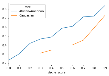
Transforming the score to percentiles by group
sufficiency_score(df_race_focused['two_year_recid'],
                  df_race_focused['decile_score'],
                  df_race_focused['race'],
                  within_score_percentile=True,
                  as_df=True).plot();
Generating all the relevant statistics for a binary prediction
report_binary(df_race_focused['two_year_recid'],
              df_race_focused['decile_score'] > 4,
              df_race_focused['race'])
| African-American | Caucasian | |
|---|---|---|
| total | 3175.000000 | 2103.000000 |
| proportion | 0.601554 | 0.398446 |
| base_rate | 0.523150 | 0.390870 |
| acceptance_rate | 0.576063 | 0.330956 |
| accuracy | 0.649134 | 0.671897 |
| fnr | 0.284768 | 0.496350 |
| fpr | 0.423382 | 0.220141 |
| ppv | 0.649535 | 0.594828 |
| npv | 0.648588 | 0.710021 |
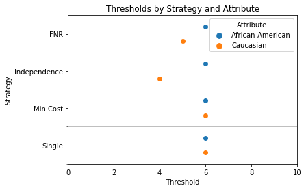
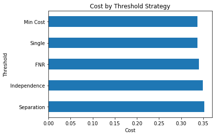
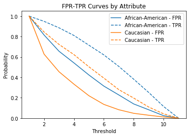
Threshold Intervention
from responsibly.fairness.metrics import roc_curve_by_attr
from responsibly.fairness.interventions.threshold import (find_thresholds_by_attr,
                                                          plot_fpt_tpr,
                                                          plot_roc_curves_thresholds,
                                                          plot_costs,
                                                          plot_thresholds)
rocs = roc_curve_by_attr(df_race_focused['two_year_recid'],
                         df_race_focused['decile_score'],
                         df_race_focused['race'])
Comparison of Different Criteria
Single threshold (Group Unaware)
Minimum Cost
Independence (Demographic Parity)
FNR (Equality of opportunity)
Separation (Equalized odds)
Cost: \(FP = FN = -1\)
COST_MATRIX = [[0,  -1],
               [-1,  0]]
thresholds_data = find_thresholds_by_attr(df_race_focused['two_year_recid'],
                                          df_race_focused['decile_score'],
                                          df_race_focused['race'],
                                          COST_MATRIX)
plot_roc_curves_thresholds(rocs, thresholds_data);